Given the Graph of the F(X) State Any Value of X Where Its Derivative Would Be Negative

Point Mobile Notice Show All NotesHide All Notes

Mobile Notice

You appear to get on a twist with a "narrow" screen width (i.e. you are probably happening a mobile earpiece). Due to the nature of the math on this site it is good views in landscape style. If your twist is non in landscape painting fashion many another of the equations will run off the side of your device (should be able to scroll to see them) and some of the menu items will be cut off attributable the narrow blind width.

Section 2-3 : Interpretations of Partial Derivatives

This is a fairly curt segment and is here so we potty acknowledge that the two main interpretations of derivatives of functions of a sole variable still hold for partial derivative derivatives, with small modifications naturally to account statement of the fact that we now have more than one variable.

The first interpretation we've already seen and is the more important of the two. As with functions of single variables partial derivatives stand for the rates of change of the functions equally the variables change. Equally we saw in the previous incision, \({f_x}\left( {x,y} \proper)\) represents the charge per unit of change of the function \(f\unexpended( {x,y} \right)\) as we change \(x\) and hold \(y\) fixed while \({f_y}\left( {x,y} \right on)\) represents the rate of transfer of \(f\left( {x,y} \right)\) as we change \(y\) and hold \(x\) fixed.

Example 1 Determine if \(\displaystyle f\left( {x,y} \right-minded) = \frac{{{x^2}}}{{{y^3}}}\) is increasing or decreasing at \(\left( {2,5} \right-handed)\),

1. if we allow \(x\) to vary and hold \(y\) regressive.
2. if we allow \(y\) to vary and hold \(x\) fixed.

Show All SolutionsFell All Solutions

a if we take into account \(x\) to vary and hold \(y\) fixed. Evince Solution

In this case we will first off need \({f_x}\leftmost( {x,y} \aright)\) and its value at the point.

\[{f_x}\left( {x,y} \right) = \frac{{2x}}{{{y^3}}}\hspace{0.5in} \Rightarrow \hspace{0.5in}{f_x}\left( {2,5} \right) = \frac{4}{{125}} > 0\]

Indeed, the uncomplete derivative with esteem to \(x\) is positive and so if we hold \(y\) leaded the function is accelerando at \(\left( {2,5} \right)\) as we alter \(x\).

b if we allow \(y\) to vary and hold in \(x\) fixed. Show off Resolution

For this part we will motivation \({f_y}\left( {x,y} \right)\) and its value at the point.

\[{f_y}\left( {x,y} \right) = - \frac{{3{x^2}}}{{{y^4}}}\hspace{0.5in} \Rightarrow \hspace{0.5in}{f_y}\left( {2,5} \right) = - \frac{{12}}{{625}} < 0\]

Here the partial with obedience to \(y\) is negative and so the routine is decreasing at \(\left( {2,5} \right)\) as we vary \(y\) and hold \(x\) fast.

Note that it is completely possible for a function to live increasing for a immobile \(y\) and decreasing for a unadjustable \(x\) at a point as this example has shown. To see a nice example of this take a look at the following graph.

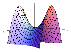
This is a graphical record of a hyperbolic paraboloid and at the bloodline we can figure that if we move in along the \(y\)-axis the graph is increasing and if we move along the \(x\)-axis the graph is decreasing. So it is wholly possible to have a chart both increasing and decreasing at a point depending upon the direction that we move. We should never expect that the function will act in on the button the synoptical way at a point as each adaptable changes.

The next interpretation was one of the standard interpretations in a Calculus I class. We know from a Calculus I class that \(f'\left( a \opportune)\) represents the pitch of the tangent line to \(y = f\left( x \right)\) at \(x = a\). Well, \({f_x}\left( {a,b} \right)\) and \({f_y}\left( {a,b} \starboard)\) besides represent the slopes of tangent lines. The difference present is the functions that they represent tangent lines to.

Partial derivatives are the slopes of traces. The biased derivative \({f_x}\left( {a,b} \ethical)\) is the pitch of the trace of \(f\left( {x,y} \right)\) for the level \(y = b\) at the point \(\left( {a,b} \right)\). Likewise the partial derivative \({f_y}\left( {a,b} \right)\) is the slope of the trace of \(f\left( {x,y} \right)\) for the plane \(x = a\) at the aim \(\left( {a,b} \right)\).

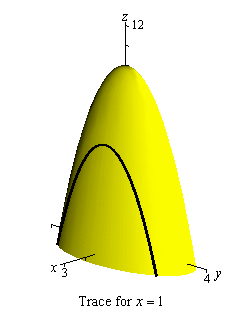
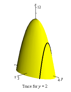
Example 2 Find the slopes of the traces to \(z = 10 - 4{x^2} - {y^2}\) at the point \(\left( {1,2} \right)\).

Show Solution

We sketched the traces for the planes \(x = 1\) and \(y = 2\) in a past section and these are the two traces for this point. For reference purposes here are the graphs of the traces.

Next, we'll need the two partial derivatives so we can get the slopes.

\[{f_x}\left( {x,y} \right) = - 8x\hspace{0.5in}{f_y}\left( {x,y} \right) = - 2y\]

To grow the slopes all we need to do is evaluate the unfair derivatives at the point in question.

\[{f_x}\left( {1,2} \right) = - 8\hspace{0.5in}{f_y}\left( {1,2} \right) = - 4\]

And then, the tan line at \(\odd( {1,2} \precise)\) for the hunt to \(z = 10 - 4{x^2} - {y^2}\) for the plane \(y = 2\) has a slope of -8. Also the tangent line at \(\socialist( {1,2} \right)\) for the trace to \(z = 10 - 4{x^2} - {y^2}\) for the plane \(x = 1\) has a gradient of -4.

Finally, get's briefly talk about getting the equations of the tangent line. Recall that the equation of a line in 3-D space is given by a vector equation. Also, to get the equation we indigence a point on the line and a vector that is parallel to the stemma.

The bespeak is unchaste. Since we know the \(x\)-\(y\) coordinates of the point wholly we need to do is plug this into the equation to cause the point. So, the point wish be,

\[\left( {a,b,f\left( {a,b} \right)} \right)\]

The parallel (or tan) transmitter is also just as easy. We can write the equating of the airfoil as a vector function as follows,

\[\vec r\left( {x,y} \right) = \left\langle {x,y,z} \right\rangle = \left\langle {x,y,f\left( {x,y} \right)} \right\rangle \]

We know that if we have a vector function of one variable we can get a tan transmitter by differentiating the transmitter function. The same will hold true present. If we differentiate with respect to \(x\) we bequeath stupefy a tangent vector to traces for the plane \(y = b\) (i.e. for fixed \(y\)) and if we severalise with respect to \(y\) we will get a tangent vector to traces for the plane \(x = a\) (operating room fixed \(x\)).

So, here is the tan vector for traces with fixed \(y\).

\[{\vec r_x}\left( {x,y} \right) = \port\langle {1,0,{f_x}\left( {x,y} \right)} \right\rangle \]

We differentiated each component with respect to \(x\). Therefore, the first component becomes a 1 and the second becomes a naught because we are treating \(y\) as a changeless when we differentiate with respect to \(x\). The third component is fitting the partial of the social function with respect to \(x\).

For traces with fixed \(x\) the tangent vector is,

\[{\vec r_y}\left( {x,y} \right) = \left\langle {0,1,{f_y}\left( {x,y} \right)} \just\rangle \]

The equating for the tangent telephone line to traces with nonmoving \(y\) is then,

\[\vec r\left( t \right) = \left\langle {a,b,f\unexhausted( {a,b} \right)} \right\rangle + t\port\langle {1,0,{f_x}\leftish( {a,b} \right)} \rightist\rangle \]

and the tangent line to traces with fixed \(x\) is,

\[\vec r\left( t \right wing) = \left\langle {a,b,f\far left( {a,b} \right)} \rightist\rangle + t\left\langle {0,1,{f_y}\left( {a,b} \right)} \right\rangle \]

Example 3 Set down the vector equations of the tangent lines to the traces to \(z = 10 - 4{x^2} - {y^2}\) at the compass point \(\left( {1,2} \right)\).

Show Solution

There really isn't all that much to practise with these other than plugging the values and function into the formulas above. We've already computed the derivatives and their values at \(\left( {1,2} \perpendicular)\) in the previous example and the point on each trace is,

\[\leftish( {1,2,f\left( {1,2} \rightfield)} \right) = \left hand( {1,2,2} \correct)\]

Here is the equation of the tangent line to the trace for the plane \(y = 2\).

\[\vec r\left( t \right) = \left\langle {1,2,2} \right\rangle + t\leftover\langle {1,0, - 8} \right\rangle = \left-handed\langle {1 + t,2,2 - 8t} \satisfactory\rangle \]

Here is the equation of the tangent dividing line to the hunt for the plane \(x = 1\).

\[\vec r\left-handed( t \right) = \leftmost\langle {1,2,2} \straight\rangle + t\nigh\langle {0,1, - 4} \right\rangle = \port\langle {1,2 + t,2 - 4t} \right-hand\rangle \]

Given the Graph of the F(X) State Any Value of X Where Its Derivative Would Be Negative

Source: https://tutorial.math.lamar.edu/Classes/CalcIII/PartialDerivInterp.aspx

Share this post